A Layperson’s Guide to the OPM: Everything You Always Wanted to Know About the OPM, But Were Afraid to Ask (Part 2)

In Part 1 of this post, we walked through the mechanics of the option pricing model (OPM) with a view to making the model more intuitive to non-specialist report users. In this post, we will address the model from a more qualitative perspective, evaluating the model’s use and potential misuse in practical application.

As promised in Part 1, we will address the following issues in this post:

• Additional economic features that can be accommodated in the OPM
• Assessing the reasonableness of required inputs and sensitivity to inputs
• Comparison of strengths and weaknesses relative to the probability-weighted expected return method
• The usefulness of the OPM backsolve method in converting per share transaction prices to an implied total equity value
• Reconciling the OPM with market participant perspectives on value

Other Economic Features That Can Be Modeled in OPM

The ComplexCo example from Part 1 included the most common economic rights (liquidation preferences, conversion features, exercise prices) found in equity instruments. The OPM can also accommodate dividends, to the extent they accumulate and affect liquidation preferences and/or conversion. Participation rights for preferred shares allow preferred shareholders to receive – in addition to their base liquidation preference – additional proceeds at liquidation on an as-if-converted basis, often up to some cap, expressed as a multiple of the liquidation preference. The mechanics of participation rights can vary modestly, but in any event can be directly modeled within the OPM framework.

More exotic, and less common, features of preferred shares include price or return hurdles that influence the allocation of proceeds to the equity holders. The OPM can also be accommodated to these features. So long, as the feature can be reduced to a function of total equity value (i.e., for a given total equity value, there is one and only one possible allocation of proceeds to the various classes), the feature can be valued within the OPM framework.

Not all features can be reduced to a function of total equity value, however. The OPM cannot be adapted to directly value differential voting rights, price protection or ratchet provisions, drag-along and tag-along rights, and pre-emptive rights. Some notable recent late-stage rounds have featured complex anti-dilution provisions, including guaranteed minimum returns in the event of an IPO that go beyond the protections offered by traditional price ratchets. When such features are present, valuation specialists need to consider whether a discrete adjustment to the results of the OPM analysis should be made in measuring fair value.

The OPM allocates the value of the existing capital structure, with the volatility parameter determining the potential changes in the value of the existing equity classes. Future issuances of additional equity are assumed to pull their own economic weight (i.e., neither contribute to, nor detract from, the value of the existing equity classes). As a result, there is no need to make assumptions in the OPM for the amount, timing, or pricing of future equity raises.

Assessing Reasonableness: Inputs

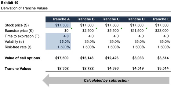
Beyond the formal elements of the capital structure that define breakpoints and tranche allocations, the required inputs to the OPM are the traditional Black-Scholes parameters. Exhibit 10 of the initial installment of this post displayed the inputs used to allocate the value of ComplexCo.

The OPM inputs can be developed, and tested for reasonableness, in the same manner as in applications of the Black-Scholes model.

• Stock Price. The stock price in the OPM is the total equity value of the subject business. The total equity value is derived through application of the traditional valuation methods under the asset-based, income and market approaches. As will be discussed in a subsequent section of this post, a known value for a particular component of the capital structure can be used to find the implied total equity value (the “back-solve” method).
• Exercise Price. The exercise prices in the OPM correspond to the equity value breakpoints identified in the formal analysis of the capital structure.
• Time to Expiration. In applying the OPM, one must assume a single point estimate for when liquidity will be achieved, either through dissolution, strategic sale, or IPO. While the actual time to expiration cannot be known with certainty, reasonable estimates can generally be made by reference to the subject company’s life cycle stage, funding needs, and strategic outlook.
• Volatility. As with time to expiration, volatility cannot be directly observed. The most common starting point for volatility analysis is an examination of historical return volatility for a group of peer public companies. If reliable data is available, implied volatility from publicly traded options on the shares of such companies may also be consulted. Analysts adjust the observed peer volatility measures to take into account life cycle stage, remaining milestones, and other qualitative factors pertaining to the subject company.
• Risk-free Rate. The risk-free rate corresponds to the assumed time to expiration.

The most challenging assumptions to establish and support in application of the OPM are the time to expiration and volatility. As discussed in the following section, testing the sensitivity of the OPM output to variation in these inputs is a critical element of assessing reasonableness.

Assessing Reasonableness: Output

We assessed the reasonableness of the OPM output from one perspective in the concluding section of Part 1 of this post. Report reviewers can quickly confirm the most basic mechanical integrity of an OPM through three easy preliminary checks: (1) the sum of the aggregate equity class allocations equals the total equity value of the subject company, (2) the sum of the fully-diluted shares used to calculate value per share equals that in the capitalization table, and (3) the rank order of the per share value conclusions is consistent with the liquidity preferences, conversion rights, and exercise prices pertinent to the various equity classes. These simple checks will not uncover all potential modelling errors, but they do eliminate a good portion of the most egregious potential pitfalls.

Beyond mere mechanical integrity, an additional step in assessing the reasonableness of the OPM output is to consider the sensitivity of the resulting allocation to changes in key inputs, principally time to expiration and volatility. Exhibit 13 provides such sensitivity analysis for ComplexCo.

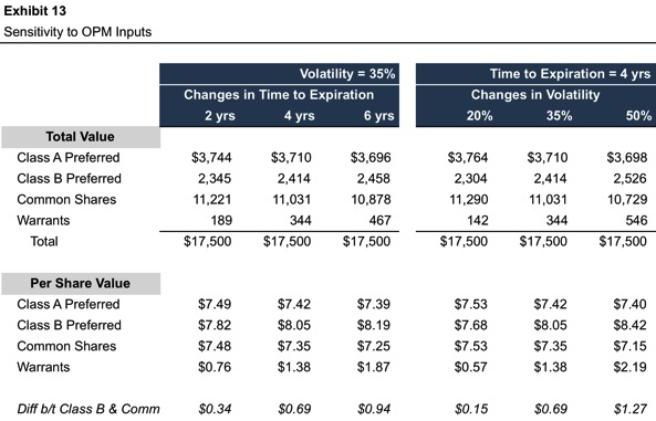
We can make a few general observations from the sensitivity analysis in Exhibit 13.

1. Since the OPM is an allocation model, the total value of the equity classes is unaffected by changes in inputs. The only impact such changes can have is on the relative allocation to various classes. This is purely a zero-sum game; for one class to increase in value, one or more other classes must decrease in value.
2. The sensitivity results are easiest to interpret for the warrants. As the junior-most security in the capital structure, the sensitivity to changes in OPM inputs is unambiguous. Increases in time to expiration cause the allocation to warrants to increase, as do increases in volatility. Furthermore, because the warrants are at the bottom of the capital stack, the sensitivity of value to changes in inputs is magnified relative to other equity classes.
3. The Class B preferred shares benefit from downside protection, as the proximity of the conversion price ($5.00) to the current common share price increases the likelihood that the liquidation preference will preserve returns to the Class B preferred shareholders. The payoff to the Class B preferred shareholders is asymmetric since the upside is unlimited through the conversion feature, while the downside is constrained by the liquidation preference. As a result, assumptions that increase the dispersion of potential future outcomes (longer time to expiration and higher volatility) cause the value of the Class B preferred shares to increase.
4. The junior preferred shares (Class A) are directionally aligned with the common shares, although the fixed liquidation preference dampens volatility relative to the common shares. In cases of short times to expiration and low volatility, the per share value for Class A approaches that of the common as the likelihood that the current share price ($7.35) will fall below the Class A conversion price ($2.00) diminishes to a trivial level.
5. The sensitivity of the common shares, which are situated between the preferred classes and the warrants, is less predictable. In this case, the warrants have a parasitic relationship to the common shares, such that increases in the value of the warrants are accompanied by decreases in common share value. This relationship does not always obtain, however; the relative proportions of the instruments in the capital structure and the “moneyness” of the various capital structure components will determine the sensitivity of the common.

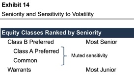
With reference to seniority, the equity classes at the “edges” of the capital structure are those that experience the greatest relative benefit from a skewed outcome. The most senior class benefits (on a relative basis) from the liquidation preference in a downside scenario, while the most junior class experiences the greatest marginal benefit from an upside scenario. Since the classes at the “edges” gain the most from skewed outcomes, they exhibit the greatest sensitivity to volatility and time factors, with the “interior” classes are less sensitive.

Strengths and Weaknesses Relative to PWERM

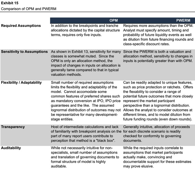
The primary analytical alternative to the OPM is the probability-weighted expected return method, or PWERM as it is affectionately known. Whereas the OPM is a continuous model, with potential future outcomes assumed to occur pursuant to a lognormal distribution, the PWERM is a discrete model which considers a finite number of analyst-selected potential outcomes and associated probabilities. In contrast to the OPM, the PWERM pulls double duty as both a valuation method and a means of simultaneously allocating the resulting value to the various equity classes.

Exhibit 15 summarizes a comparison of the two models along a variety of axes.

Reliability of Backsolve Application of OPM

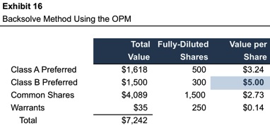
The OPM is not a valuation method. However, if the value of any component of the capital structure is known – through either a contemporaneous primary issuance or secondary trade – the enterprise value corresponding to that value can be determined. Using the OPM to work backward from output to an indication of implied total equity value is known as the “backsolve” method.

As an example, consider the case of ComplexCo at the time the Class B preferred shares were issued at a price of $5.00 per share (one year prior to the valuation date in our Part 1 example). What was the implied total equity value of the company at that time? By starting with the known value of $5.00 per Class B preferred share, we can work backward, developing estimates for all the other assumptions, to determine the implied total equity value. In this case, we conclude that all assumptions are unchanged from Exhibit 10, with the exception of time to expiration, which is five years, instead of four. As shown in Exhibit 16, the resulting total equity value is $7,242 at the issuance date, compared to $17,500 at the later valuation date from our prior example in Part 1 of this post.

This procedure is reasonable and appropriate in many circumstances. In our experience, however, it is important to keep in mind how the limitations of the OPM (primarily the lognormal distribution of outcomes) can distort the results of the analysis. When reading “backwards” from the value of a single equity class to the value of all equity, the effect of such distortions can be magnified. In our experience, the potential magnitude of such distortion is greatest when the known value is for the most senior security in the capital structure. In many cases, the lognormal assumption causes total loss scenarios to be under-represented in the probability distribution of potential future outcomes relative to market participant expectations. When combined with the use of the risk-free rate in a risk neutral framework, the OPM may assign greater value to the liquidation preference than market participants do. This can cause the difference between the most senior preferred class and other components of the capital structure to be exaggerated, resulting in an understated total equity value.

In our view, these distortions can be further aggravated when the equity class used to calibrate the total equity value accounts for only a small portion of the subject company’s capital structure. In our practice, we temper the effect of this issue by also giving weight to the total equity value which is the product of the known per share price and the fully-diluted share count.

Reconciling the OPM with Market Participant Perspectives

There is an irony at the heart of fair value measurement. Fair value is, by definition, a market participant concept. In other words, a “correct” fair value measurement will reflect the exit price for the subject asset among a group of relevant market participants. However, some techniques for measuring fair value are rarely, if ever, used by actual market participants.

In our experience working with market participants in early-stage companies, new financing rounds are generally priced through a two-step process: (1) negotiate the pre-money total equity value of the company, and (2) divide that figure by the fully-diluted share count. These market participants clearly understand that the economic rights associated with senior preferred shares are valuable. However, they do not develop or express a discrete estimate of that value. We suspect that there are at least two potential explanations for this. First, the economic rights that benefit the senior preferred shares may be the required “sweetener” to arrive at the headline total equity value. Second, in many early-stage companies, the actual benefit of a liquidation preference may be perceived as limited. Certainly, the scenario that would trigger payout of a liquidation preference, in lieu of participating as common shareholder following conversion, is sub-optimal. If the most likely outcomes are smashing success (in which case everyone converts and is treated equally) or abysmal failure (in which case being first in line to get nothing is not helpful), market participants may be less impressed by the economic rights accruing to the senior securities than the OPM would seem to be.

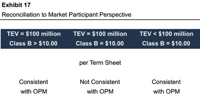
Assuming we are right, this perfectly rational behavior on the part of market participants can put those with the responsibility to measure fair value in a difficult spot. Consider a company that recently closed a $20 million Class B round, with customary liquidation preferences and conversion rights. The term sheet states that the pre-money equity value is $100 million. There are 10 million Class A preferred and common shares outstanding, and the issuance price for the Class B round is $10 per share.

As shown in Exhibit 17, there are three logical possibilities in this case. The only case that is inconsistent with the OPM is the one that reflects the actual, stated terms of the transaction.

There is no simple solution to this conundrum. However, to our mind it does underscore the appropriate posture toward analytical tools like the OPM. The fair value measurement tool should serve the market participant perspective; the market participant perspective should not be subordinated to the fair value measurement tool, no matter how insightful and “correct” it may be. As we have recently noted, Fidelity reports identical per share values for different equity classes of a given investee company. In doing so, one is effectively disregarding the differential economic rights of the various classes. Strictly speaking, such a conclusion is economically untenable. Yet, it likely mirrors how Fidelity, and other market participants, actually view value.

Conclusion

Use of the OPM in fair value measurement is growing. The model has many attractive attributes, including its precision, small number of assumptions, muted sensitivities, and auditability. However, the model is not necessarily appropriate in all circumstances. The underlying assumption of lognormality may not be appropriate for some companies, and may limit the usefulness of the backsolve technique for determining implied total equity values. In our view, the model is best used in conjunction with the PWERM. Finally, as with all fair value measurement models, valuation specialists should carefully evaluate the degree to which the results of the model cohere with the market participant perspective.

Related Links

• Marking Illiquid Investments in Liquid Funds
• Preferences and FinTech Valuations
• Unicorn Valuations: What’s Obvious Isn’t Real, and What’s Real Isn’t Obvious
• Consequences of Calcified Cap Charts: A Few Thoughts on Startup Equity-Based Compensation