Community Bank Valuation (Part 4): Valuing Minority Interests

In the June 2019 BankWatch we began a multi-part series exploring the valuation of community banks. The first segment introduced key valuation drivers: various financial metrics, growth, and risk. The second and third editions described the analysis of bank and bank holding company financial data with an emphasis on gleaning insights that affect the valuation drivers. We now conclude our series by assembling these pieces into the final product, a valuation of a specific bank.

While it would streamline the valuation process, there is no single value for a bank that is applicable to every conceivable scenario giving rise to the need for a valuation. Instead, valuation is context dependent. This edition of the series focuses on the valuation of minority interests in banks, which do not provide the ability to dictate control over the bank’s operations. The next edition focuses on valuation considerations applicable to controlling interests in banks that arise in acquisition scenarios.

Valuation Approaches

Valuation specialists identify three broad valuation approaches within which several valuation methods exist:

1. The Asset Approach develops a value for a bank’s common equity based on the difference between its assets and liabilities, both adjusted to market value. This approach is less common in practice, given analysts’ focus on banks’ earnings capacity and market pricing data. In theory, a rigorous application of the asset approach would require determining the value of the bank’s intangible assets, such as its customer relationships, which introduces considerable complexity.
2. The Market Approach provides indications of value by reference to actual transactions involving securities issued by comparable institutions. The obvious advantage of this approach is the coherence between the goal of the valuation itself (the derivation of market value) and the data used (market transactions). The disadvantage, though, is that perfectly comparable market data seldom exists. While we will not cover the topic in this article, transactions in the subject bank’s common stock, which often occur for privately held banks due to their frequently widespread ownership and stature in the community, may serve as another indication of value under the market approach.
3. The Income Approach includes several methods that convert a cash flow stream (such as earnings or dividends) into a value. Two broad subsets of the income approach exist – single period capitalization methods and discounted cash flow methods. For bankers, a single period capitalization is analogous to a net operating income capitalization in a real estate appraisal; it requires an earnings metric and a capitalization multiple. Alternatively, bank valuations often use projection-based methodologies that convert a future stream of benefits into a value. The strengths and weaknesses of a projection-based methodology derive from a commonality – it requires a forecast of future performance. While creating such a forecast is consistent with the forward-looking nature of investor returns, predicting the future is, as they say, difficult.

The following discussion focuses on the valuation methodologies used most commonly for banks, the comparable company method and the discounted cash flow method.

Comparable Company Method

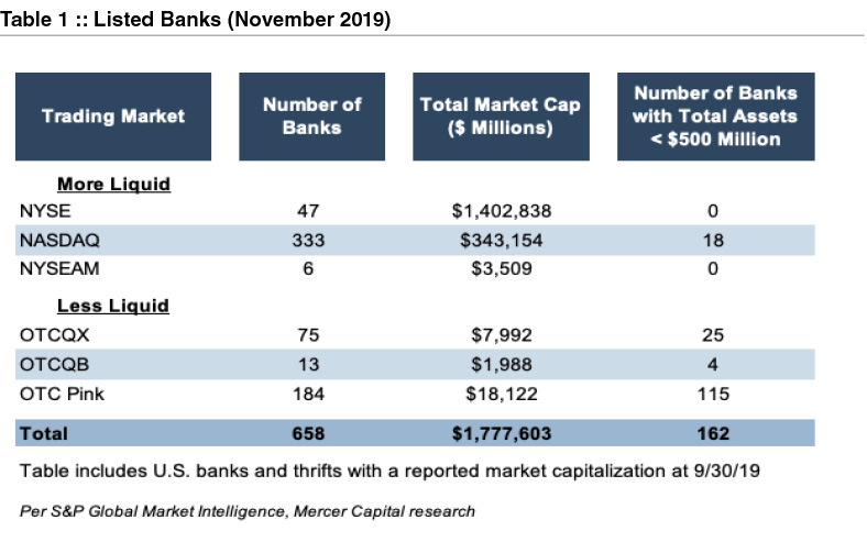
Bank analysts are awash in data, both regarding banks’ financial performance but also market data regarding publicly traded banks’ valuation. Table 1 presents a breakdown by trading market of the number of listed banks in November 2019.

To narrow this surfeit of comparable company data, analysts often screen the publicly traded bank universe based on characteristics such as the following:

• Size, such as total assets or market capitalization
• Profitability, such as return on assets or return on equity
• Location
• Asset quality
• Revenue mix, such as the proportion of revenue from loan sales or asset management fees
• Balance sheet composition, such as the proportion of loans or dependence on wholesale funding
• Trading market or volume

Even after applying screens similar to the preceding, it remains doubtful that the publicly traded banks will exactly mirror the subject bank’s characteristics. This is especially true when valuing smaller community banks, as a relatively limited number of publicly traded banks exist with assets of less than $500 million that trade in more liquid markets. Ultimately, the analyst must determine an appropriate valuation multiple based on the subject bank’s perceived growth opportunities and risk attributes relative to the public companies. For example, analysts can compare the subject bank’s historical and projected EPS growth rates against the public companies’ EPS growth rates, with a materially lower growth outlook for the subject bank suggesting a lower pricing multiple.

Part 1 of this community bank valuation series described various valuation metrics applicable to banks, most prominently earnings and tangible book value. It is important to reiterate that while bankers and analysts often reference price/tangible book value multiples, the earning power of the institution drives its value. Chart 1 illustrates this point, showing that price/tangible book value multiples rise along with the core return on tangible common equity. This chart includes banks traded on the NASDAQ, NYSE, or NYSEAM with assets between $1 and $10 billion.

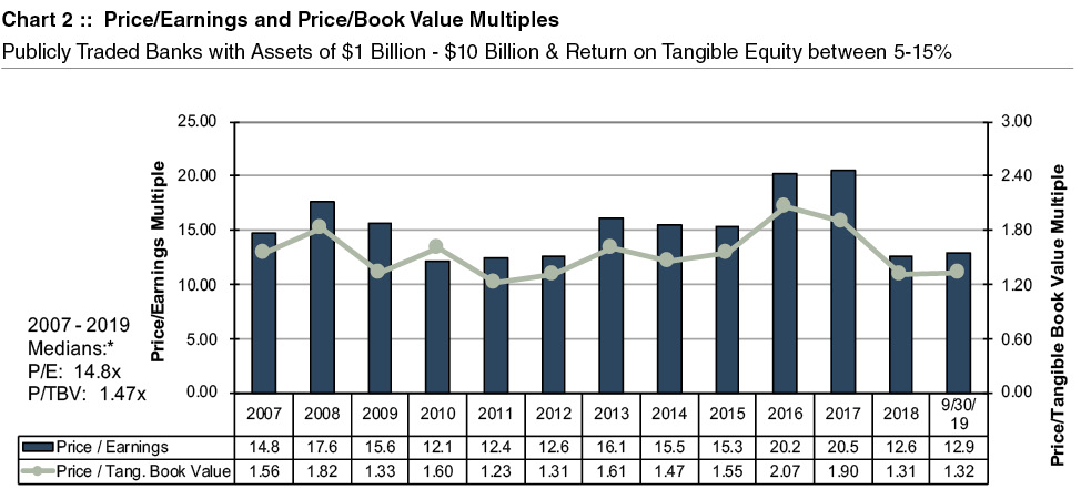
Since banking is a more mature industry, bank price/earnings multiples tend to vary within a relatively tight range. Chart 2 provides some perspective on historical price/earnings and price/tangible book value multiples, which includes banks traded on the NASDAQ, NYSE, or NYSEAM with assets between $1 and $10 billion and a return on core tangible common equity between 5% and 15%. Trading multiples in the first several years of the analysis may be distorted by recessionary conditions, while the multiples reported for 2016 and 2017 were exaggerated by optimism regarding the potential, at that time, for tax and regulatory reform. The diminished multiples at yearend 2018 and September 30, 2019 reflect a challenging interest rate environment, marked by a flat to inverted yield curve, and the possibility for rising credit losses in a cooling economy.

Discounted Cash Flow Method

The discounted cash flow (DCF) method relies upon three primary inputs:

• A projection of cash flows distributable to investors over a finite time period » A terminal, or residual, value representing the value of all cash flows occurring after the end of the finite forecast period
• A discount rate to convert the discrete cash flows and terminal value to present value

1. Cash Flow

First, a few suggestions regarding projections:

• For a financial institution, projecting an income statement without a balance sheet usually is inadvisable, as this obscures important linkages between the two financial statements. For example, the bank’s projected net interest income growth may require a level of loan growth not permitted by the bank’s capital resources.
• Including a roll-forward of the loan loss reserve illustrates key asset quality metrics, such as the ratios of loan charge-offs to loans and loan loss reserves to loans. The level of charge-offs should be assessed against the bank’s historical performance and the economic outlook.
• Key financial metrics, both for the balance sheet and income statement, should be assessed against the bank’s historical performance and peer banks.
• While projections can be prepared on a consolidated basis, we prefer developing separate projections for the bank and its holding company. This makes explicit the relationships between the two entities, such as the holding company’s reliance on the bank for cash flow. For leveraged holding companies, a sources and uses of funds schedule is useful.

In preparing a DCF analysis for a bank, the most meaningful cash flow measure is distributable tangible equity. The analyst sets a threshold ratio of tangible common equity/tangible assets or another regulatory capital ratio based on management’s expectations, regulatory requirements, and/or peer and publicly traded comparable company levels. Equity generated by the bank above this target level is assumed to be distributed to the holding company. After determining the holding company’s expenses and debt service requirements, the remaining amount represents shareholder cash flow, which then is captured in the DCF valuation analysis.

2. Discount Rate

For a financial institution, the discount rate represents the entity’s cost of equity. Outside the financial services industry, analysts most commonly employ a weighted average cost of capital (WACC) as the discount rate, which blends the cost of the company’s debt and equity funding. However, banks are unique in that most of their funding comes from deposits, and the cost of deposits does not rise along with the entity’s risk of financial distress (because of FDIC insurance). Therefore, a significant theoretical underpinning for using a WACC – that the cost of debt increases along with the entity’s risk of default – is undermined for a bank. Analytical consistency is created in a DCF analysis by matching a cash flow to equity investors (i.e., dividends) with a cost of equity.

A bank’s cost of equity can be estimated based on the historical excess returns generated by equity investments over Treasury rates, as adjusted by a “beta” metric that captures the volatility of bank stocks relative to the broader market. Analysts may also consider entity-specific risk factors – such as a concentration in a limited geographic market, elevated credit quality concerns, and the like – that serve to distinguish the risk faced by investors in the subject institution relative to the norm for publicly traded banks from which cost of equity data is derived.

3. Terminal Value

The terminal value is a function of a financial metric at the end of the forecast period, such as net income or tangible book value, and an appropriate valuation multiple. Two techniques exist to determine a terminal value multiple. First, the Gordon Growth Model develops an earnings multiple using (a) the discount rate and (b) a long-term, sustainable growth rate. Second, as illustrated in Chart 2, bank pricing multiples tend to vary within a relatively tight range, and a historical average trading multiple can inform the terminal value multiple selection.

Correlating the Analysis

In most analyses, the values derived using the market and income approaches will differ. Given a range, an analyst must consider the strengths and weaknesses of each indicated value to arrive at a final concluded value. For example, earnings based indications of value derived using the market approach may be more relevant in “normal” times, as the values are consistent with investors’ orientation towards earnings as the ultimate source of returns (either dividends or capital appreciation). However, in more distressed times when earnings are depressed, indications of value using book value assume more relevance. If a bank has completed a recent acquisition or is in the midst of a strategic overhaul, then the discounted cash flow method may deserve greater emphasis. We prefer to assign quantitative weights to each indication of value, which provide transparency into the process by which value is determined.

Relative Value Analysis

The analysis is not complete, however, when a correlated value is obtained. It is crucial to compare the valuation multiples implied by the concluded value, such as the effective price/earnings and price/tangible book value multiples, against those reported by publicly traded banks. Any divergences should be explainable. For example, if the bank operates in a market with constrained growth prospects, then a lower than average price/earnings multiple may be appropriate. A higher return on equity for a subject bank, relative to the comparable companies, often results in a higher price/tangible book value multiple. As another reference point, the effective pricing multiples may be benchmarked against bank merger and acquisition pricing to ensure that an appropriate relationship exists between the subject minority interest value and a possible merger value.

Conclusion

There are many valuation issues that remain untouched by this article in the interest of brevity, such as the valuation treatment of S corporations and the discount for lack of marketability applicable to minority interests in banks with no active trading market. Instead, this article addresses issues commonly faced in valuing minority interests in any community bank. A well-reasoned valuation of a community bank requires understanding the valuation conventions applicable to banks, such as pricing multiples commonly employed or the appropriate source of cash flow in a DCF analysis, but within a risk and growth framework that underlies the valuation of all equity instruments. Relating these valuation parameters to a comprehensive analysis of a bank’s financial performance, risk factors, and strategic outlook results in a rigorous and convincing determination of value. In the next edition, we will move beyond the valuation of minority interests in banks, focusing on specific valuation nuances that arise when engaging in a valuation for merger purposes.

Originally published in Bank Watch, November 2019.

About the Author