The following is an installment in our series “What Keeps Family Business Owners Awake at Night”.
Successful family businesses are built over time, and building well requires investment. Since a given dollar of cash flow generated by a business will either be returned to capital providers or reinvested in the business, a company’s reinvestment policy is essentially the inverse of its distribution policy: businesses that reinvest heavily will make modest distributions, while those that emphasize large distributions will have less available for reinvestment in the business.
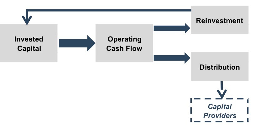
Cash distributed leaves the business, providing current returns to investors, while reinvested funds remain in the business with the expectation that the retained capital will generate returns which contribute to capital appreciation. In other words, the tradeoff between current return and capital appreciation is rooted in the corresponding tradeoff between distribution and reinvestment.
For a family business, investment can take different forms.
- Capacity maintenance and modernization. Tangible assets wear out, and technological advances can render existing assets inefficient relative to available replacement assets. It may be possible to defer certain expenditures with few observable consequences in the short-term, but the bill always comes due eventually. While investments in capacity maintenance and modernization are not always the most exciting, successful family businesses recognize their priority for long-term sustainability.
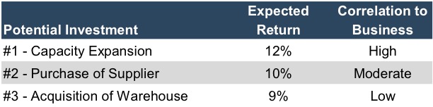
- Capacity Expansion. In our experience, businesses are either growing or dying – holding steady is nearly impossible over the long-term. Investments in capacity expansion help keep family businesses on a growth footing. Depending on the company’s circumstances, growth investments may involve penetrating new geographic markets, introducing new product lines, or research to develop products for an unmet market need.
- Acquisitions. Rather than building incremental capacity, managers and directors of a family business may determine that it is more efficient to assimilate existing industry capacity through an acquisition. Acquisitions offer the opportunity to “hit the ground running” with a built-in customer base, workforce, tradename and other intangible assets that typically accrue slowly over time. On the other hand, acquisitions present integration and culture challenges (and the risk of overpayment) not relevant to other forms of investment. For perspective, during the most recent year, the companies in the S&P 600 small cap index spent $24.2 billion on acquisitions, compared to $28.7 billion on capital expenditures, with nearly 40% of the companies having completed at least one acquisition.
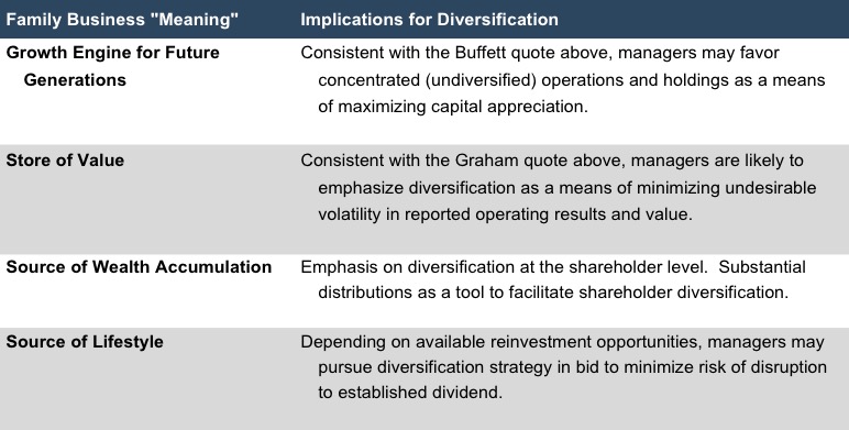
- Diversification. Acquisitions are often classified as either vertical (purchase of a supplier or customer) or horizontal (purchase of a competitor). Both types of acquisitions have some organic connection to the existing business. Sometimes, however, family businesses make investments that are unrelated to legacy operations. It is not uncommon for family businesses to make investments for the sake of diversification, particularly as the business matures and the number of shareholding generations increases.
One of my favorite Seinfeld moments (among many) is set at the car rental counter, where an exasperated Jerry explains to the uncomprehending agent the difference between taking a reservation and holding a reservation. Taking the reservation is easy, but holding the reservation is what really matters. In the same way, investing for growth is easy: there are plenty of equipment dealers eager to sell shiny new machines and investment bankers who can’t wait to describe an exciting acquisition target. But making good investments – those for which the tradeoff between current returns and capital appreciation worthwhile – is considerably harder. So, what are the marks of a good investment?
- Market opportunity. A good investment addresses an identifiable need in the market. Further, given the competitive environment in the relevant markets, the identified need can be met profitably. In other words, management should have a simple and straightforward answer to the threshold question: Why does this make sense?
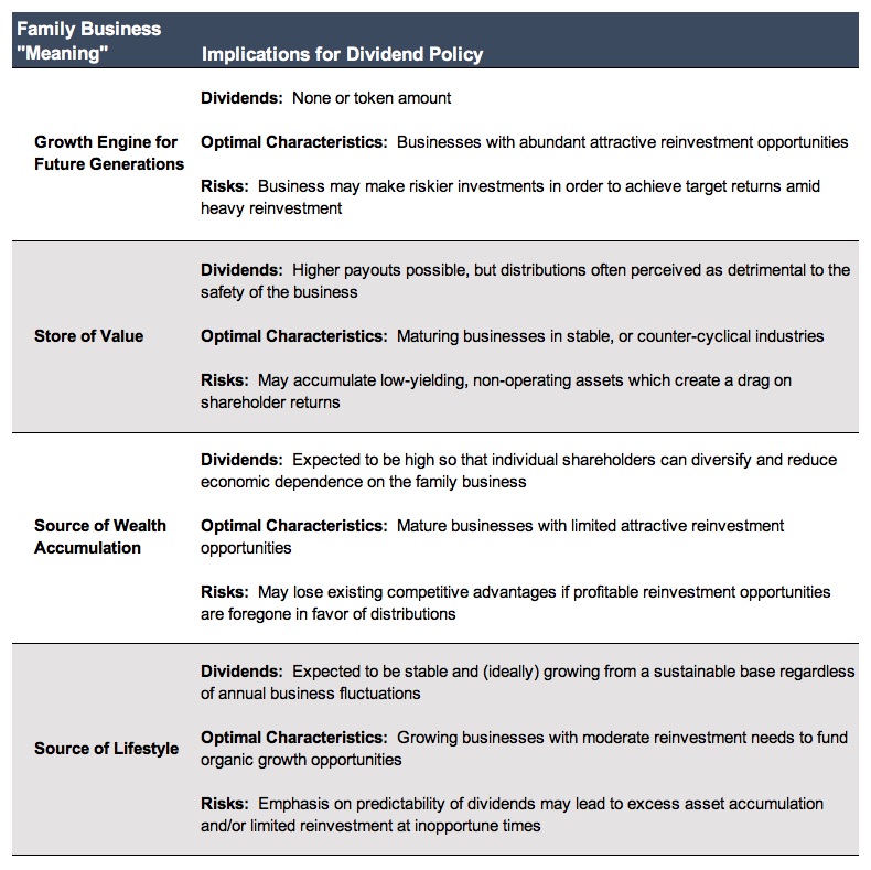
- Strategic fit. Family business managers and directors should also have a concise and credible answer to the natural follow-up question: Why does this make for us? In other words, how does the proposed investment complement the company’s corporate strategy? If it extends or deviates from the current strategy, why is the strategy adjustment appropriate? As we described in the context of distribution policy, the business can have a variety of potential “meanings” to the family – does the proposed investment cohere with the “meaning” of the family business?
- Financially vetted. A thorough capital budgeting process will involve calculating relevant return measures (internal rate of return, net present value) to assess whether the investment opportunity is likely to increase or decrease the value of the company. Of course, figures lie and liars make spreadsheets. For a proposed investment that addresses a real market opportunity and is a strategic fit for the company, the financial vetting process should be geared to answering another vital question: What financial results are necessary for this investment to be good for us? Has management assembled a compelling case for the expected returns, or is the investment more of a “trust me” exercise?
- Plan for monitoring. The most often neglected component of the capital budgeting process is establishing a feedback mechanism for the investment. Too often, capital investments simply melt away into the general corporate asset pool, with no reliable means of evaluating whether the investment generated an appropriate return. In other words, how will we know if this investment was, in fact, good for us? The ability to evaluate past investments is critical to making better investments in the future.
All family businesses need to evaluate how they are investing for future growth. Managers and directors must navigate carefully between the risks of depressed future returns through over-investment (i.e. empire building) and losing existing competitive advantages through insufficient reinvestment. The long-term sustainability of the family business depends on it.
 For more information about Mercer Capital’s core deposit services, please contact us.